
Excel’s IFERROR function traps errors that are returned from a formula or calculation. It gives you control over what is returned instead of an error message, such as IFERROR then blank.
Links to topics on this page
- Errors captured by IFERROR
- IFERROR() function – definition and arguments
- Excel IFERROR then blank
- IFERROR with VLOOKUP
- IFERROR perform another function
For example, instead of a formula returning Excel’s default ‘#N/A’ error, you might want to:
- IFERROR then blank, i.e. return no text at all, or
- VLOOKUP and return specific text, e.g. use with VLOOKUP to return “Value not found”;
- perform a different function or formula.
IFERROR() checks for the following errors:
#N/A, #VALUE!, #REF!, #DIV/0!, #NUM!, #NAME?, #NULL!.
A valid answer will be returned as normal if there is no error.
IFERROR Excel definition
=IFERROR( result [you enter your formula/function here], value_if_error )
IFERROR() arguments
- result = value resulting from a function / formula / calculation; you enter your formula/function here to be checked in the IFERROR function;
- value_if_error = the value or instruction you specify for Excel to return if ‘result‘ is an error;
- If the function / formula / calculation returns a valid answer, its result is returned as normal.
Syntax – plain English definition
=IFERROR( Formula/calculation to be checked for errors [result will be returned if no error], Value/formula/calculation to be returned if there is an error )
IFERROR then blank – syntax
=IFERROR( A2/B2 , “” )
The example above calculates the formula ‘A2 divided by B2’ (i.e. cell contents of A2 and B2), and if this results in an error, the result returned is a blank cell. If A2/B2 produces a valid result it is returned as normal.
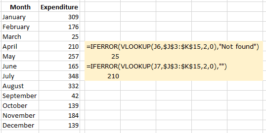
IFERROR and VLOOKUP – syntax
=IFERROR( VLOOKUP ( G4,$B$2:$D$26,3,FALSE ) , “Value not found” )
The above example performs a lookup for a value (in cell G4) in a range ($B$2:$D$26) in column 3, and if the value is not found, then the string “Value not found” is returned.
The VLOOKUP function is wrapped inside an IFERROR() function.
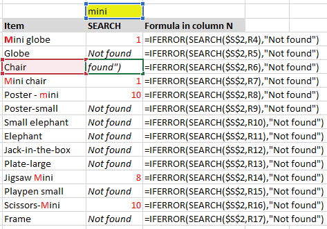
See our post here on how to use the SEARCH function with IFERROR https://excelquick.com/excel-function/search-specific-text-sum-values/.
See our other posts on VLOOKUP:
- VLOOKUP examples
- VLOOKUP MATCH – two-way lookup
- VLOOKUP with CONCATENATE
IFERROR then perform another function – example
=IFERROR( I8/J8 , I8/$M$4 )
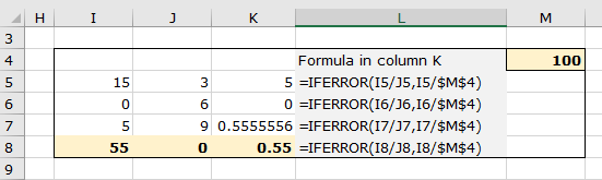
In the example above, the calculation in row 8, I8/J8 (55 divided by 0) results in an error, so the second formula (I8/$M$4) is calculated instead.