Purpose

To apply a conditional formatting rule in Excel to non-adjacent cells.

Links to topics on this page

• Video of method 1: create a conditional formatting rule and apply the rule to other cell ranges
• Method 1 steps: apply conditional formatting to non-adjacent cell ranges
• Method 2: copy and paste formatting

---

Syntax — enter non-adjacent ranges in the ‘Applies to‘ field for the conditional formatting rule

= L4:L13, M4:M13, N4:N15, O4:O15

Video — create a conditional formatting rule to highlight values, then copy the rule to other non-adjacent cells

---

Method 1 (steps shown in video above) — apply conditional formatting to non-adjacent cells

1. Click the first cell, or range of cells, that the conditional formatting is to be applied to.
2. Create the formatting rule and click OK.
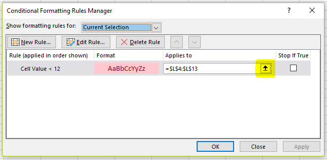
3. With the cursor still in the cell or range, select Conditional formatting | Manage rules, for ‘Current selection‘ (screenshot at top of page).
4. Click the range icon next to the rule, and the first cell or range you selected will be highlighted.
5. Add a comma after the first selection, and now select the next cell or range that you want to add.
6. Keep adding more selections with a comma in between each.
7. When done make sure your last selection is not followed by a comma (or your selections will be lost and you will have to start again).
8. Click OK.

Key point

Use a comma to separate the non-adjacent cells/ranges in the selection field.

Watch out for

Don’t add a comma at the end of the selection, otherwise, when you apply the change, your selections will be lost and you will need to reselect.

Method 2 — copy and paste with formatting

Another method is to simply copy and paste with formatting.

• Select and copy the cell or range of cells that you wish to take the conditional formatting from.
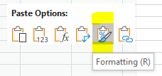
• Select the destination cell or range of cells, right-click and select the ‘Formatting‘ icon. This will paste just the formatting not the cell value.
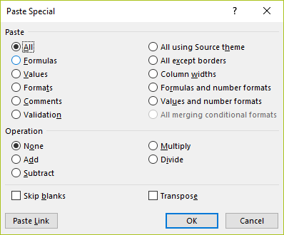
• Or, you can open the ‘Paste special‘ dialog box from the home tab of the ribbon, and make a selection.