How to create a macro to sum a column of data
Creating macros in Excel can be so quick and easy. Macros are super helpful to automate common tasks, reducing the amount of clicks and keystrokes that we need to make.
In this example we’re going to:
- first build the FORMULA that we want to automate,
- and then create a MACRO to run the formula.
Links to topics on this page
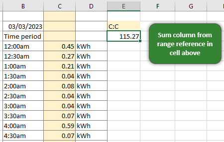
EXAMPLE We have long columns of data which we want to sum, and instead of having to scroll to the bottom of the column, and summing from there, we want a macro to return the total for us. We want to choose where on our spreadsheet the total value will appear, and we want the column of figures to be able to vary, so we can add new values, or paste in a whole new set of values.
 Another trick we’re going to use is a dynamic reference with the INDIRECT() function to choose which column we get the total for.
Dynamic formula to get the value from the cell above
To make our macro more helpful than summing one specific column of data, we want to make it more dynamic by being able to:
- vary the column range to sum, and
- easily be able to place the total value anywhere we want on the worksheet / in the workbook.
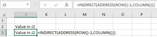
We therefore need a formula which will ‘read the value from the cell above‘, and the value will be a column reference (e.g. A:A specifies column A, B:B column B, etc.).
This is how we return the value from the cell above, and use the value as a cell reference:
=INDIRECT(ADDRESS(ROW()-1,COLUMN()))INDIRECT()reads the value from a cell as a cell reference (e.g. A2, C14)ADDRESS(ROW()-1,COLUMN())is the formula to reference the cell above (one row up -1, same column).
Formula to sum the column referenced in the cell above
To sum the column taking a column reference from the cell above, we wrap our relative reference above inside the SUM() function AND add a second INDIRECT() because we’re using the returned value as a range reference. The right-hand INDIRECT() gets the value from the cell above, and the left-hand INDIRECT() feeds the value into the SUM() function as a cell range reference.
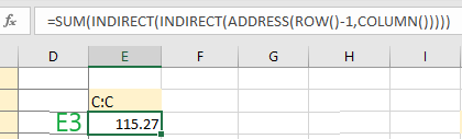
=SUM(INDIRECT(INDIRECT(ADDRESS(ROW()-1,COLUMN()))))Create a macro to sum a column
We’re now ready to create our macro. Here are the steps to create the macro which will sum any column of values that we specify. We will be able to run the macro by clicking in the cell directly below the cell where we have typed the column reference.
- Copy the SUM(INDIRECT(…) formula reference above into Notepad to make it easy to paste into your macro
- Enter a column reference in a cell on your worksheet – e.g. enter
C:Cinto cell E2 - Click in the cell below >> E3
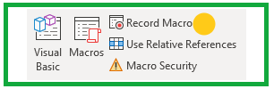
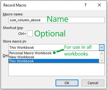
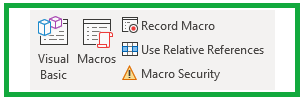
- On the Developer tab, click ‘Record Macro‘
- Enter a name for the macro, select a location where to store the macro, and optionally set a keystroke shortcut and give a description.
- Close the dialog box by clicking OK.
- Now copy the formula you’ve got ready in Notepad, and paste it into the formula bar for E3
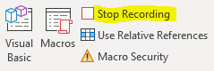
- Click on ‘Stop Recording‘. Your macro is complete and ready to use!
Run a saved Macro from the macro dialog box
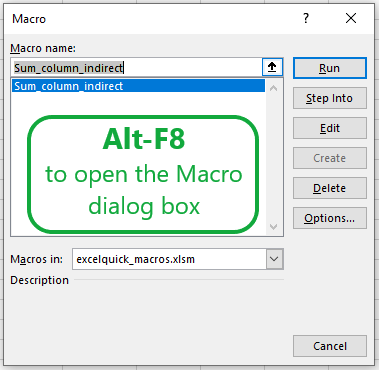
To view, run and edit saved Macros, press Alt-F8 to open the macro dialog box. Or open via the ‘Macros‘ button on the Developer tab in the ribbon.
To RUN the desired macro:
- first, click in the cell where you want the macro to be actioned.
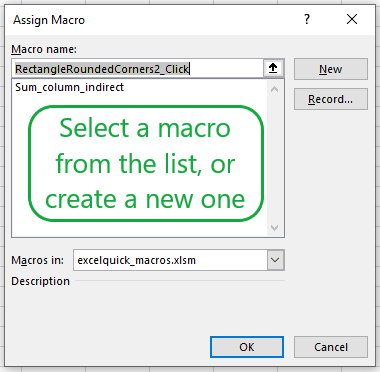
- Then open the macro dialog box with Alt-F8, select the macro from the list, and click ‘Run’.
Create a button for your Macro
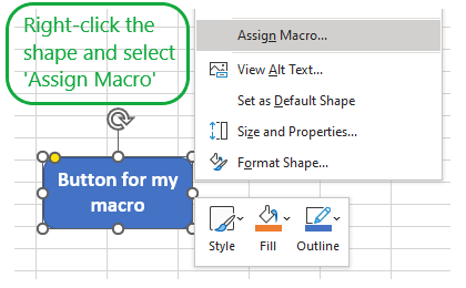
The easiest way to create a button for your macro is to:
- create a simple shape element (Insert – Shape)
- format it how you’d like, and
- then assign a macro to it: right-click, and select
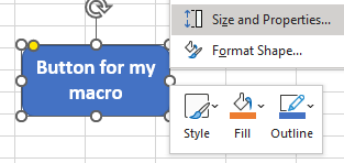
Assign Macro... - You can also set the button’s size and properties to set its position on the worksheet.
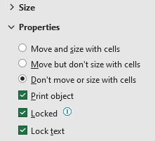
You can also add a button from the Control / Forms toolbox, but there are fewer options for styling the button compared to using a simple shape element.
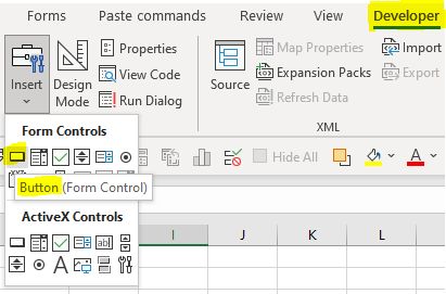
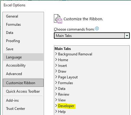
Enable the Developer tab on the Excel ribbon
The Developer tab on Excel’s ribbon isn’t showing by default, but it’s easy to switch it on through Excel’s general options.
- Go to
File | Optionsand thenCustomize Ribbon - Select
Main Tabsfrom the ‘Choose commands from:’ dropdown - And then click on Developer and Add.