How to use the Excel INDIRECT function – use text in a cell to create a cell reference
Links to topics on this page
- Basic example – read a cell reference from text
- Use INDIRECT to reference cells in other worksheets – build worksheet+cell references
- Worked example – create a summary sheet
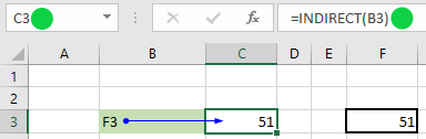
Basic example: INDIRECT – read a cell reference from text in a cell
This is the basic method of how INDIRECT() works:
- enter a cell reference as text in one cell (e.g. as in the screenshot above, enter ‘F3’ into cell B3, where you want to CREATE the cell reference),
- enter
=INDIRECT(B3)into cell C3, where you want to pull the value held in the cell reference TO - enter the value in F3 – the cell you want to REFER TO (to get the final output value from)
- C3 will now pull the value from cell F3 (51). C3’s formula is
=INDIRECT(B3), output value = 51.
| Cell | Cell content |
|---|---|
| B3 | F3 |
| C3 | =INDIRECT(B3) [output = 51, the content of cell F3) |
| F3 | 51 |
Although the INDIRECT function appears to be a very simple method, it has a lot of powerful uses to enable complex referencing, flash filling, and absolute and relative cell referencing.
INDIRECT can also be used to change cell references used within formulas without having to edit formulas themselves, just update the cells which contain the referencing.
The above example shows how to enter a cell reference as text, but …
… INDIRECT will also evaluate sheet names and file paths entered as text into cell references. See the example below.
Use INDIRECT to reference cells in other worksheets
=INDIRECT(C$3&”!$D$2″)
This uses a combination of:
- C$3 the cell from which the cell reference is extracted
- “!$D$2” text inside quotes which will be evaluated ‘as-is’:
- the quotes denote the contents to be read as text
- the exclamation mark defines the preceding text as a sheet name
- the $D$2 specifies the absolute cell reference for cell D2.
Excel INDIRECT function worked example – create a summary sheet
In the example below we want to collate data from multiple worksheets into a summary sheet, using the Excel INDIRECT function to quickly build the cell references.
In this example, we have student exam records, one student per worksheet.
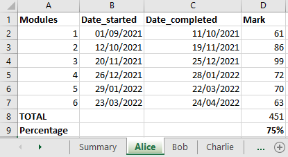
In our summary sheet we just want to pull in some headline data from each student, using cell referencing.
 Note that our column names in the summary table match the worksheet names.
 - Also, all the tables in our student worksheets have the same layout, so cell D2 in worksheet
Alice!is her mark for Module 1, and cell D2 onBob!is his mark for Module 1.
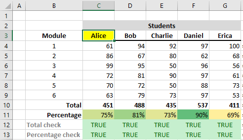
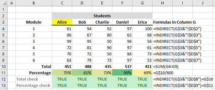
By using INDIRECT() in the cell referencing, we can more efficiently create the summary table using flash fill. We’re going to use the student names entered into row 3, columns C:G inside our INDIRECT formulas.
We just need to enter the INDIRECT formulas into the first column of the summary table, and then we can drag-fill to populate the whole table.
The ‘direct’ cell reference for Alice’s mark for Module 1 (cell $D$2 on the worksheet named Alice) is =Alice!$D$2. The table below shows how to create this cell reference using INDIRECT(). We use a combination of the cell reference (the cell that contains the sheet name), plus a string (text) inside quotes that INDIRECT will read in as-is.
| ‘Direct’ cell reference | Cell reference using Excel INDIRECT function |
|---|---|
| =Alice!$D$2 | =INDIRECT(C$3&”!$D$2″) |
| Cell C3 contains the text ‘Alice’ (the worksheet name) & symbol joins (concatenates) the cell reference and the string “!$D$2” is the remainder of the full worksheet+cell reference and we wrap that in quotes "" so that INDIRECT evaluates the characters as-is.Remember to add the exclamation mark ! after the sheet name. |
- We use the absolute reference $D$2 (absolute column absolute row) for the cell on the student worksheet because we don’t want that to change when we drag-fill the formula.
- We use C$3 (relative column absolute row) for the cell that we’re getting the worksheet name from.
- When we drag-fill the formula ACROSS the row of the summary table, it will update to D$3, E$3 etc. (change the column index but not the row number);
- and as we drag-fill DOWN the column of the summary table, the column index and the row number will stay the same.
We can copy the formula down column C under the Alice header, and just need to amend each row number in the D column cell references $D$3, $D$4, $D$5 etc.
This is what the formulas look like in column G, to fill the values from Erica’s worksheet. This updated automatically to create the correct references when we dragged the formulas across the rows.
 See our post on the basics of referencing cells in Excel: absolute and relative cell referencing in Excel.
Verifying the cell referencing – quick check
To check that we’re bringing in the correct values from each sheet, we’re calculating the totals and percentages on the summary sheet, and then using conditional formatting to check the summary sheet totals with the totals on each worksheet.
The error returned if an invalid reference is used is #REF!.
See more on Microsoft’s support page.