How to use Excel INDIRECT with INDEX MATCH lookups
Links to topics on this page
- Excel’s INDIRECT function
- INDEX MATCH basic formula
- INDIRECT INDEX MATCH worked example
- Tips on using INDIRECT with INDEX MATCH
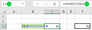
Excel’s INDIRECT function evaluates text as cell references:
=INDIRECT(B3)
… where B3 contains a cell reference (e.g. F3)
… and B3 can contain other reference elements such as worksheet name / file path, using the ‘&’ symbol to join string elements to create a full worksheet+cell reference.
=INDIRECT(B3&”!$C$4″)
 See our topic where we demonstrate how to use Excel’s INDIRECT function to set up static cell references, to quickly build a summary table of data from multiple worksheets.
In the article on this page, we show how to combine INDIRECT with INDEX MATCH to create dynamic cell referencing, and make data collation more efficient and robust.
INDEX MATCH basic formula
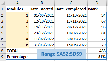
- We have student exam records in a workbook, one worksheet per student.
- Six exam modules 1-6 can be taken in any order.
- The student scores are contained within the range $A$2:$D$9 on each sheet, but the module order listed in the table rows may differ.
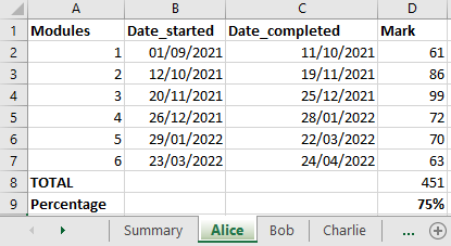
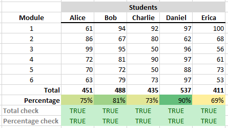
- We want a summary sheet as shown below that collates the marks for each student.
- A lookup will refer to the correct row for each module on the student worksheets.
- Dynamic cell references will make it quick to create the table.
- Note that the summary table headings for the students match the worksheet names.
In this worked example we’re going to use INDEX MATCH.
The basic formula for INDEX MATCH is:
=INDEX(range, MATCH(lookupValue, columnRange, matchType), colNum)
![]() See our post here on how to use INDEX MATCH: https://excelquick.com/excel-function/index-match/
See our post here on how to use INDEX MATCH: https://excelquick.com/excel-function/index-match/
The static INDEX MATCH formula we need to look up Bob’s mark for Module 1 is shown below:
=INDEX(Bob!$A$2:$D$9,MATCH($B4,Bob!$A$2:$A$9,0),4)
Components of the INDEX MATCH formula above:
- Bob!$A$2:$D$9 – INDEX absolute range A2:D9 on worksheet named Bob
- MATCH the value in cell $B4 on the summary sheet (contains ‘1’ for module 1)
- Bob!$A$2:$A$9,0 – Look up the value ‘1’ in absolute column range A2:A9 on worksheet Bob; 0 designates an exact match is required
- Find the value we want in column 4 (D) of the index range (A2:D9), which is 94, Bob’s mark for Module 1.
If we use the static references we’d have to copy paste and edit each formula.
Instead, we use the INDIRECT function to create dynamic worksheet+cell references. We will look up the correct rows on each student’s worksheet, and will be able to drag-copy the formulas in the summary table. We can also use INDIRECT to read in the INDEX and MATCH ranges, because each student worksheet has the same layout.
Excel INDIRECT INDEX MATCH worked example
See above for the description of the example task we’re using to demonstrate using Excel’s INDIRECT function with INDEX MATCH.
We’re using INDIRECT to read the worksheet name, and the INDEX and MATCH cell ranges. As you can see below, here’s how the formula will combine INDEX MATCH and INDIRECT:
=INDEX (INDIRECT (worksheet name! + index range), MATCH (module number, INDIRECT (worksheet name! + match range), matchType), column number).
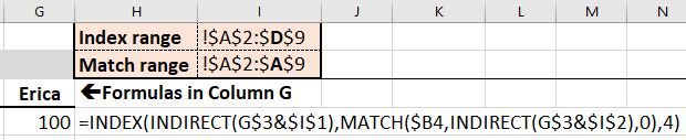
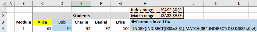
- We reference the worksheet name! from the summary table heading row (C3 to G3 in the screenshots below).
- We’ve entered the INDEX and MATCH cell ranges into cells I1 and I2.
- Note we included an exclamation mark at the beginning ‘!’ of the cell ranges to denote the preceding text as a sheet name.
=INDEX(INDIRECT(D$3&$I$1),MATCH($B4,INDIRECT(D$3&$I$2),0),4)
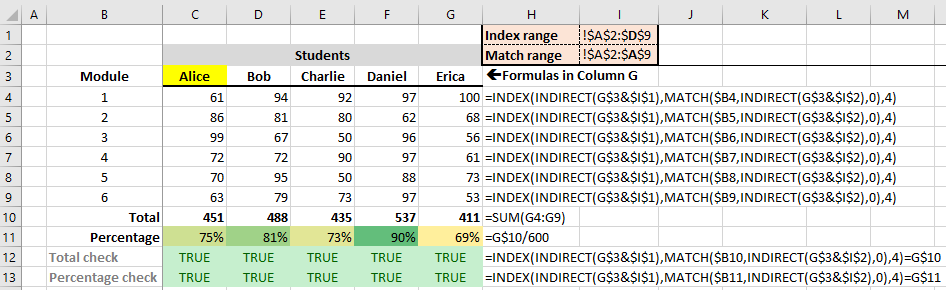
Here below is how the INDIRECT INDEX MATCH formulas look in Column G of the summary table, to bring in Erica’s results.
We’ve also built in some validation checks to confirm that the totals and percentages in the summary table match the worksheet calculations.
 Note that if we need to change the cell ranges for the lookups, all we need to do is amend the values entered into cells I1 and I2 and all the formulas in the summary table will update automatically.
Tips on using Excel’s INDIRECT function
- Using the method in this article, work out the static INDEX MATCH formula first before working out how to use INDIRECT for the cell referencing.
- Make use of absolute and relative cell referencing to make it easy to drag-fill formulas in a summary table – see our topic here on the basics of using absolute and relative cell referencing.
- Create checks to validate your referencing. For example, here we’ve calculated totals and percentages on the summary page, and then checked that they match the values on the individual worksheets.