
How to look up values using INDEX and MATCH in Excel
AIM: Look up a value in one column based on the value in another column by combining Excel’s INDEX and MATCH functions.
Topics on this page
- VLOOKUP vs INDEX MATCH
- Syntax – INDEX function
- INDEX and INDEX MATCH examples
- INDEX example – single column range (list, or vector)
- INDEX example – 2-column range (array)
- Syntax – MATCH function
- Syntax – INDEX MATCH
- INDEX MATCH example
VLOOKUP vs INDEX MATCH
Although Excel’s VLOOKUP function is very powerful, one main limitation is that you can only look up a value in the first column of a range of cells and look to the right of that column – you can’t look up a value in column 2, and find the target value to the left in column 1. However, with INDEX MATCH in Excel you can look either to the left or to the right.
Syntax – INDEX function in Excel
=INDEX(range, rowNum, colNum)
Excel’s INDEX function finds a value in a range of cells, where:
- range defines the range of cells to look in,
- rowNum = row number (in the range), and
- colNum = column number (in the range).
KEY NOTE: It’s important to understand that the row and column numbers refer to the range, not to the worksheet row and column numbers.
INDEX and INDEX MATCH examples
INDEX example – single column range (list, or vector)
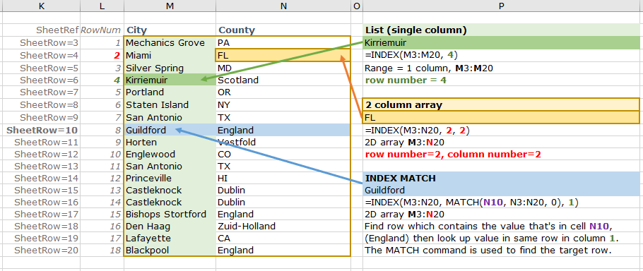
=INDEX(M3:M20, 4) [INDEX(range, rowNum]
…defines the single column range M3 to M20, and returns the value in row 4 (of the cell range M3:M20, which will be worksheet cell reference M6).
INDEX example – 2-column range (array)
=INDEX(M3:N20, 2, 2) [INDEX(range, rowNum, colNum]
…defines the two-column range (array) M3 to N20, and finds the value in row 2 and column 2 (of the range M3:N20, which is worksheet cell reference N4).
Syntax – MATCH function in Excel
=MATCH(lookupValue, range, matchType)
- lookupValue = known value to look up
- range = cell range to look in (column or row)
- matchType = 0 (FALSE) or 1 (TRUE), where 0/FALSE means ‘find the exact match‘, and 1/TRUE means ‘find the nearest approximate match‘.
Syntax – INDEX MATCH in Excel: use MATCH to find the target row to look in
=INDEX(range, MATCH(lookupValue, columnRange, matchType), colNum)
INDEX MATCH uses the MATCH function to tell the INDEX function which row to look in (i.e. INDEX solves [MATCH(lookupValue, columnRange, matchType)] and uses that value as the rowNum argument).
INDEX MATCH example in Excel
=INDEX(M3:N20,MATCH(N10,N3:N20,0),1)
[INDEX(range, rowNum(=the row that contains the value in N10), colNum]
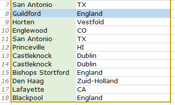
…defines the two-column range M3:N20, finds the value that is in cell N10 in the range N3:N20 [in this example, row 8 in the range], then looks in column number 1 in row 8. In this example, shown in the screenshot above, there are several instances of the value in N10 (England), and Excel will stop looking when it finds the first match in the range.