
- VLOOKUP Syntax – Excel definition
- Description
- Method
- Quick test – spot the potential error!
Excel’s VLOOKUP function is one of the key functions to learn in Excel, and once used you’ll wonder how you ever did without it!
Purpose
- VLOOKUP is a ‘vertical’ lookup which looks up a value in one column, and moves along the row to find a second value in another column.
- VLOOKUP aims to look up data organised in rows, where each row is a new record.
- The common use for this function is looking up a set of values from one table (range of cells) to fill in a column of values in another range.
- E.g. find city names for a list of customers by looking up values in an address table.
Syntax – Excel definition
=VLOOKUP(value, range, column_index, [range_lookup])
Syntax – simple definition
=VLOOKUP(The known value, The range to look in, The column number in which to look up the second value, Match the first value approximately or exactly)
Syntax – example
=VLOOKUP($A2,$E$2:$K$24,5,FALSE)
Description
-
- In the example above, the value in cell A2 is being looked up in a row in column E, and the value returned is in the same row, in the 5th column; the match must be exact (because FALSE is used at the end of the formula).
- e.g. if this was an example to look up a city name for a customer:
- VLOOKUP(CustomerName, AddressTable, 5, FALSE) – where ‘5’ is the column number, and ‘FALSE’ requires an exact match
- $A2 contains the customer name
- $E$2:$K$24 is the range of cells (address table) to look in.
- In Excel’s technical definition [range_lookup] means ‘match type’.
- See a second example in the screenshot below – see if you can spot a potential mistake!
Method
- Type the formula in the cell where you want the looked up value to be entered.
- Double-click the right hand corner of the cell to send the formula down the column to the last row containing data.
- Use absolute cell references in the range so that when you copy the formula to another cell, the same range of cells is going to be looked in.
Watch out for
- The column which contains the known value (customer name) MUST be in the first column of the lookup range. This means that it HAS to be to the left of the column looked in to return the second value (a potential limitation for the uses of VLOOKUP).
- The default match type is approximate, so use ‘FALSE’ at the end of the formula for an exact match (as in example above).
Useful tips
- Use named ranges / tables with VLOOKUP – you can add extra rows and columns to the range being looked up, and the table will automatically expand to include the new values – and the VLOOKUP formula won’t need to be changed because a table name has been used.
VLOOKUP example – spot the potential error!
- The formula in Cell C15 will create an error if it is copied down the column … can you spot what it is? Have a look again at the Method above.
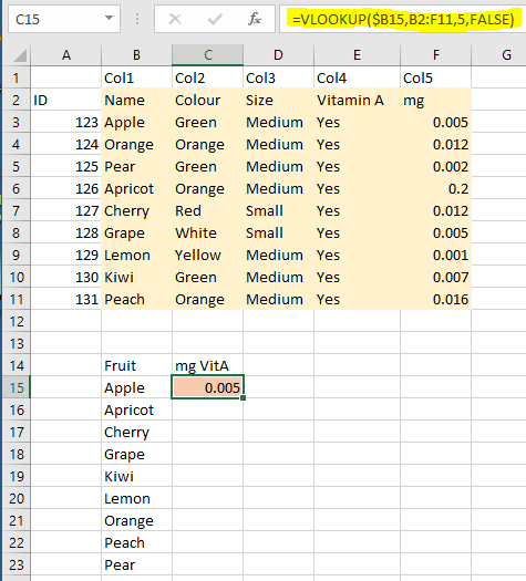
The range B2:F11 referenced in the formula is relative not absolute. If the formula is dragged down the column, the range will be changed relative to the starting range. It no longer refers back correctly to the desired range. The correct form of the range to use is: $B$2:$F$11.