Purpose

Remove blank cells in a list of values in Excel, retaining the original list.

Method

Use Excel’s Advanced Filter on the Data tab | Sort & Filter section.

The example below copies the values to a new column. This helps if your original list is part of a table or matrix, and you want to retain the original records/rows in the table.

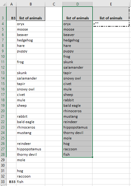
• Column B contains the list to remove blanks from. For this method, the list needs to include a header. The list in column B will be filtered to only include cells that contain a value (i.e. greater than nil/null, defined by:  >””  [greater than symbol followed by two speech mark symbols]).
• Column D is the destination column where the values will be copied to. Make sure to leave a blank column in between if your original list is part of a defined table (otherwise the new column will be automatically added to the table, and amend the original).
• Column E holds the ‘criteria’ by which the original values will be filtered.

1. Copy the header (‘list of animals’) from the original list (Col B) to the top of the destination range(Col D), and to a second range top cell(Col E).
2. Type >”” into the cell under the header in the second column (Col E, in this example cell E4).
3. Select the range to be filtered, including its header (B3:B33, click and drag to highlight the cells).
4. Click on ‘Advanced filter’ in Data | Sort & Filter.
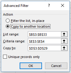
5. In the dialogue box:
   • select ‘Copy to another location‘.
   • Confirm that the range in the List range field is the range of your list (B3:B33).
   • Next to the Criteria range field, click on the up arrow and select the header and criteria cells (E3:E4), click OK.
   • Next to the Copy to field, click on the up arrow and select a range of cells in the destination column (Col D), including the header cell and long enough to take the list of filtered values.
   • Click OK.
6. The filtered list of values with no blanks will appear in the destination column, (Col D).

Notes

• You can also use the ‘Unique records only‘ option if your list has duplicates, and you want to just retain the unique values.
• In the example above, the top cells of the columns were being used for explanatory notes. The method works fine for any range – at the top of columns, or further down.
• Microsoft Excel’s error messages in the Advanced Filter dialogue box can be somewhat unhelpful. I found the key to this working was to make sure that each of the three ranges has the same heading at the top.
• This method could be used to filter for other criteria, e.g. wildcards, particular values.