
Purpose: to find a value in a table by looking up row and column values
Links to topics on this page
- VLOOKUP in Excel
- Syntax: basic VLOOKUP
- Key note about VLOOKUP
- Combining VLOOKUP MATCH in Excel for a two-way lookup
- Syntax: VLOOKUP MATCH
- Key note about VLOOKUP MATCH
- Basic VLOOKUP MATCH example
VLOOKUP in Excel
The VLOOKUP function in Excel enables you to look up values in a column, based on the value in the same row in another column.
Syntax: basic VLOOKUP
=VLOOKUP(value, range, column_index, [range_lookup])
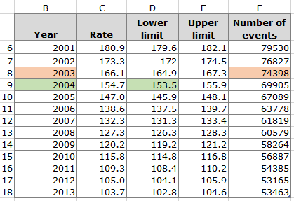
For example, in the table above, we can get Excel to find value ‘74398‘ in column F, by first finding the value ‘2003‘ in the column B, and then looking for the value in the same row in column F. The formula for this would be:
=VLOOKUP(“2003”, $B$6:$F$18, 5, 0)
- where “2003” is the value to look up
- $B$6:$F$18 is the cell range to look in; column B is column #1, and column F is #5
- 5 is the column number to look in
- 0 is the match type.
Key note about VLOOKUP
The key thing to remember about the VLOOKUP function is that the column where the known value is being looked up HAS to be in the left hand (first) column of the range being looked in. In our example above, we can only look up in column B (because we have defined the range to include columns B to F). If we ask Excel to look for a known value in column C (using the range B to F), the VLOOKUP won’t work.
RELATED POST: See the basic VLOOKUP method explained in detail on our topic page here: https://excelquick.com/excel-function/vlookup-excel-function/ .
Combining VLOOKUP MATCH in Excel for a two-way lookup
Combining the VLOOKUP and MATCH functions in Excel, uses the MATCH function to specify which column to look in. There are different options on how to configure the MATCH statement, and one option can create a dynamic lookup for the column reference.
Syntax: VLOOKUP MATCH
=VLOOKUP(ROWValueToLookUp, Range1 [whole range], MATCH(COLUMNValueToLookUp, Range2 [to find the column value], MatchType [for the MATCH function), MatchType [for the VLOOKUP function])
Key note about using VLOOKUP and MATCH
The two ranges Range1 and Range2 have to start with the same cell reference in the top left hand position.
Basic VLOOKUP MATCH example
Let’s start with a simple example of using VLOOKUP with MATCH in Excel to find a value.
Syntax: VLOOKUP and MATCH example with hard-coded value
=VLOOKUP(“2003”, $B$5:$F$18, MATCH(“Number of events”,$B$5:$F$5,0),0)
Syntax example explanation
In the formula above:
- “2003” is the known value to find in column B
- $B$5:$F$18 is the whole range to look in; it must contain the column headings where we’re going to specify the column value to look up
- “Number of events” is the known value to find in the column headings (row B5 to F5), and specifies which column for Excel to return the target value
- the first 0 is the match type for the MATCH function (to find the exact match)
- the second 0 is the match type for the VLOOKUP function
- NOTE that the two ranges (B5:F18, and B5:F5) both start with B5 in the top left hand position
- the value returned will be 74398 from column F.