
Purpose: To apply conditional formatting based on dates falling in the current week
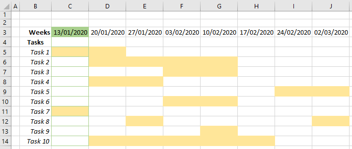
For example, we have a Gantt chart where we want to highlight the current week:
Syntax: check for dates falling in the current week
=WEEKNUM(CellRef) = WEEKNUM(NOW())
In the example Gantt chart above, we want the cells in Row 3 to highlight green when the date falls into the current week. We set up the conditional formatting rule as below.
- highlight the cells C3 to J3 (the range that the rule will apply to, and this can be updated after the rule has been set up),
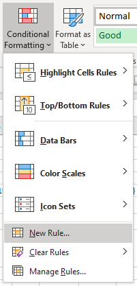
- select ‘Conditional formatting | New rule‘ from the ‘Home’ tab on the ribbon,
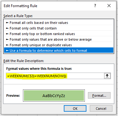
- and select the option ‘Use a formula to determine which cells to format‘
- enter the formula below:
=WEEKNUM(C$3) = WEEKNUM(NOW())
We use a mixed cell reference (C$3):
- no $ symbol before the column label (C) so that the conditional formatting rule will check in the relevant column; this will change relative to the starting column C, and
- $ symbol before the cell number label (3), so that it will only refer to the values in row 3.
We apply two separate rules using the SAME FORMULA, but with different formatting styles, so that we can apply:
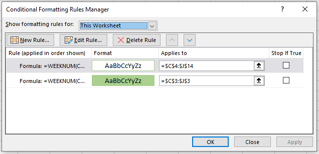
- solid green fill to the week date in row 3, and
- green borders to the cells down the column (so we don’t overlay the yellow fills which are showing the task ranges).