
Purpose: to create, rename and format Excel Tables.
Creating an Excel Table turns a simple grid or matrix of data into a structured object which has many useful properties.
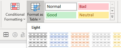
The ‘Format as Table‘ options are on the Home tab of Excel’s ribbon, next to the ‘Conditional Formatting’ options.
Links to topics on this page
- 10 benefits to using tables in Excel
- To format a range of cells as a table
- Resize an Excel Table
- Rename a table in Excel
- Add ‘Change Table Name’ to the Quick Access Toolbar
- To add totals and other summary data and functions to a table in Excel
- Using a form for data entry into a table
10 benefits to using Tables in Excel
- A table in Excel automatically expands when new rows or columns are added, so formulas or charts referencing the table will update dynamically;
- Easy to create a pivot table — click in any cell in the table, and select Insert | Pivot table from the ribbon;
- Add slicers — you may be familiar with using slicers with pivot tables; you can also use them in tables. Select ‘Insert slicer‘ from the Table Design tab in the ribbon;
- Auto-filling columns — change the formula in any cell, and the whole column will update (with the easy option to NOT auto-populate the column if you don’t want it);
- Totals and other summary functions are easy to add (see details below);
- Use a data entry form to add data (see details below);
- Structured referencing makes it easier to build, read and check formulas;
- There are lots of styles to choose from the style selector, and table styling automatically updates as the table expands. It’s also easy to change the style of the whole table, or create your own custom style;
- Ranges within the table are automatically named;
- Sorting and filtering are automatically activated in an Excel Table.
To format a range of cells as a table
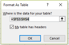
- Select the range of cells to be turned into a table.
- Select ‘Format as Table‘ from the Home tab in the ribbon.
- In the dialog box that opens, tick the box ‘My table has headers‘ if your range of cells contains a column header row. If you don’t already have column headers, Excel will automatically add ‘Column1’, ‘Column2’, ‘Column3’, etc. You can easily amend column headers.
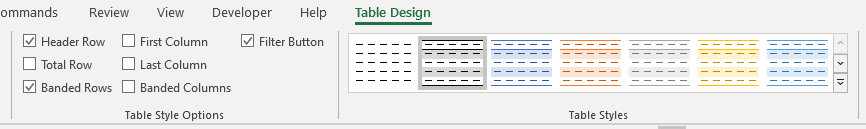
- Select the desired styling from the table design options.
When a table is created or being amended, the ‘Table Design‘ tab in Excel’s ribbon will automatically appear.
If you paste data into a worksheet in Excel, the range is highlighted, and you can select ‘Format as Table’ straightaway, without having to re-select the data (very helpful with a large set of data).
Resize an Excel Table
An Excel Table will automatically add new rows and columns as you add new data adjacent to the existing table boundaries.
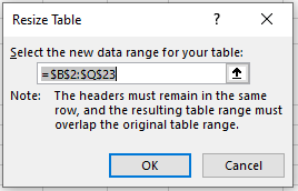
However, you may wish to make manual adjustments to the table, which you can do via the ‘Properties‘ section on the ‘Table Design‘ tab on the ribbon.
Select ‘Resize Table‘ from Properties, and the Resize Table dialog box opens. An adjustable border surrounds the existing table, and the new range can be set via the Select new data range box.
Note that Excel alerts you to the fact that the headers must remain in the same row, and the resulting table range must overlap the original table range (i.e. contain at least some of the header row and cell range of the existing table).
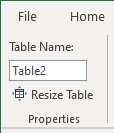
Rename a table in Excel
When tables are created, Excel will automatically name them ‘Table1’, ‘Table2’, ‘Table3’ etc.
Rename tables to something more useful via the ‘Properties‘ section of the Table Design tab of Excel’s ribbon.
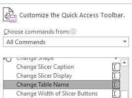
Customize the Quick Access Toolbar in Excel to include the ‘Change Table Name’ command
Right-click ‘Table Name’ in the ‘Properties’ section of the Table Design tab, and select ‘Add to Quick Access Toolbar‘. If you’re working with several tables within a workbook, it’s handy to always be able to view the name of the current table you’re working in.
You can also add it to the list of commands, and place it in the order you want in the QA toolbar, via the ‘Customize the Quick Access Toolbar’ options.
See more options on customizing the ribbon in Excel in our topic page.
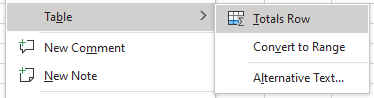
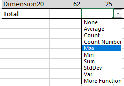
To add totals and other summary data and functions to a table in Excel
- Right-click any cell in the table, and select Table | Totals Row.
- An additional row will be added to the bottom of the table, and each column can be summarized (total, average, count, min, max, etc.) using the dropdown arrow in the bottom cell.
Using a form for data entry into a table
- Note: the ‘Form’ command in Excel isn’t on the ribbon by default, so you’ll need to add it — see our page on how to customize the ribbon in Excel.
- Select ‘Form‘ from the ribbon or Quick Access Toolbar.
- See our page on how to create a data entry form in Excel and enter or amend data.