Purpose: sum values in a range of cells based on whether another range contains specific text

Summary of steps on this page

• Use Excel’s SEARCH function to look for specific text in a range of cells
• Convert the SEARCH results into TRUEs and FALSEs using ISNUMBER
• Use the TRUE and FALSE values to then sum the values. Two options:
  • using SUMIF
  • using SUMPRODUCT

---

Excel’s SEARCH function

Syntax – SEARCH()

= SEARCH( text_to_find, within_text, [start_number])

SEARCH() function arguments

• text_to_find = the string of text to search for
• within_text = the cell reference of the text (string) to look in
• start_number (optional) = the position number of the character in the target string to start looking from.

Excel’s SEARCH function returns the position number of where the first character in the search string appears in the target string.

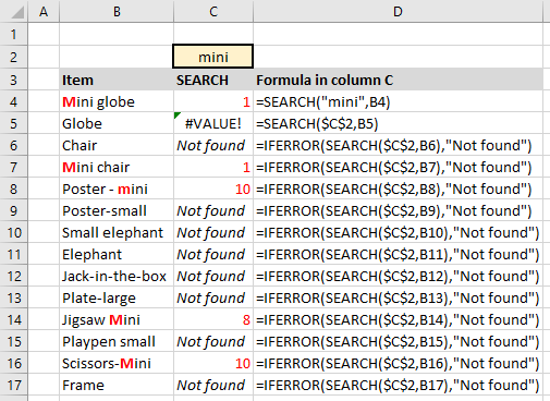
See examples below:

• You can search for a hard-coded string (e.g. “mini”), or a cell reference containing the text to search for (cell reference $C$2 in the example shown below);
• If the target cell does not contain the search text, Excel returns a #VALUE! error. To return a more ‘user friendly’ result than the #VALUE! error, you can wrap the SEARCH function in an IFERROR statement to return “Not found” if the cell does not contain the search text.
• SEARCH is NOT case sensitive. To search for case sensitive text, use Excel’s FIND function.

---

Worked example

Using the SEARCH function shown above, sum the values in column I, based on whether the Items in column H contain the text string “mini”

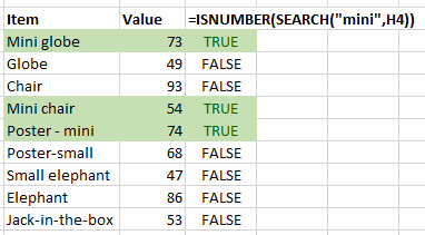
Turn the results of the SEARCH function into TRUE/FALSE values using ISNUMBER

In order to specify which values to sum from column I, it will be more helpful to have ‘TRUE/FALSE’ values returned from the SEARCH() function, rather than the start position number of the search string.

We know that SEARCH() returns a number if the text is found, or an error message if the text is not found. Therefore, we can simply test whether or not the result of the SEARCH() function is a number, using ISNUMBER().

Syntax – search for text and return TRUE if found, or FALSE if not found

=ISNUMBER( SEARCH (“text_to_find”, cell_ref))

Use SUMIF to sum the values based on the SEARCH for specific text

Syntax – SUMIF

=SUMIF(range_to_look, criteria, [range_to_sum])

• where range_to_look = the range to look in;
• criteria = criteria you specify, e.g. numeric or text values to check against;
• range_to_sum (optional) = range of values to sum which can be different to the range you ask Excel to check the criteria in.

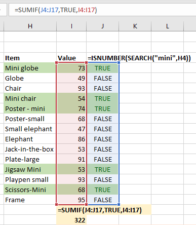
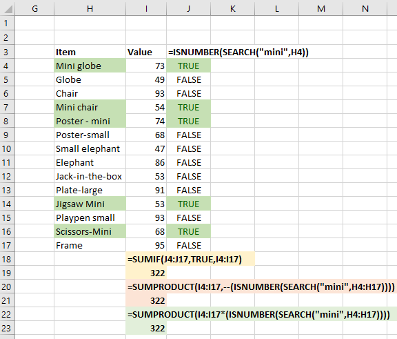
We can use Excel’s SUMIF function to sum the values in column I if the values in column J are ‘TRUE’. In this method, we’re using two separate formulas in the two columns I and J, because we can’t wrap the ISNUMBER and SEARCH formulas inside SUMIF.

However, another method uses SUMPRODUCT and combines the two steps into one, see below:

Use SUMPRODUCT to sum the values based on the SEARCH for specific text

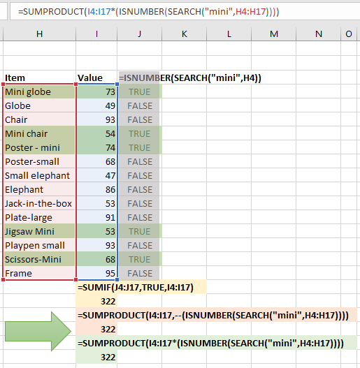
We wrap our ISNUMBER and SEARCH formulas inside a SUMPRODUCT() function.

We just need to make one small adjustment by adding either a double dash ‘–‘, or asterisk ‘*’ before the ISNUMBER formula to turn the TRUEs and FALSEs into 1’s and 0’s; SUMPRODUCT can use these values to determine which values to sum.

We therefore don’t need the separate formulas in column J to create this sum of values based on the specific text in column H.