
Purpose: create a dynamic array of values in Excel, which will update automatically as the source table changes
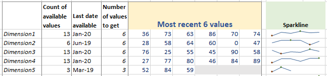
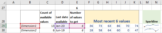
Table of latest values linked to a source data table
Links to sections on this page
- Description of the worked example
- Overview of steps to retrieve the dynamic array
- Step 1: Format the source table as an Excel Table
- Step 2: Find out the number of values available for each variable
- Step 3: Get the column header of the last value in the row
- Find the last non-empty cell in a row
- Step 4: Retrieve a dynamic array of the latest n values
- Excel’s OFFSET() function – syntax, examples and explanation
- Note about array formulas and Excel versions
- Full dynamic array formula explained
- Step 5: Plot the values in a sparkline chart
- Excel functions and features used to create a dynamic array of values
- Related topics
Worked example – get an array of latest values from a raw dataset:
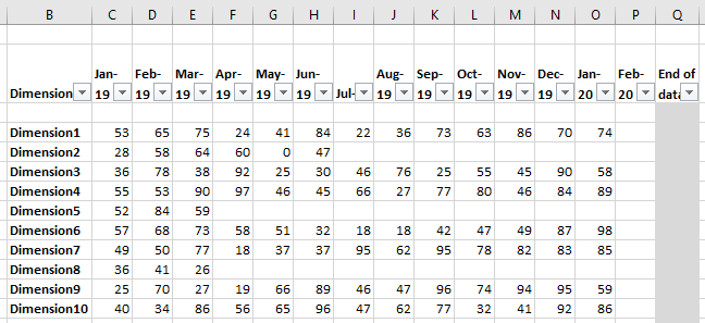
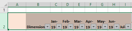
- We have a table of values for a list of variables (labelled ‘Dimensions‘ in our table shown below) which we will be adding new values to over time. This is our ‘source‘ data table.
- Not all variables have values for every month.
- As we add more columns to the table over time, it will become more fiddly to navigate, so we want to set up a separate table where we retrieve a dynamic array of the latest values.
- This new table will automatically update as new values are added to the source table.
- We will plot the latest values in a sparkline chart.
Source data table from which the latest values are retrieved
Steps to retrieve the latest set of values from the source data table:
- Step 1: Format the source table as an Excel Table;
- Step 2 :Find out the number of values available to retrieve for each variable;
- Step 3: Find out the column header of the latest value available, the last cell in the row containing a value;
- Step 4: Get a dynamic array of the latest values;
- Step 5: Plot the values in a sparkline chart.
Step 1: Format the source table as an Excel Table
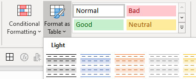
Excel Tables are structured objects which make it easier and more efficient to manipulate, analyse, sort and format data.
The ‘Format as Table‘ options are found on the Home tab of Excel’s ribbon.
To turn a matrix of values into an Excel Table:
- highlight the cells containing your data;
- select ‘Format as Table‘ from the ribbon;
- choose styling options, and rename the table from the Table Design tab;
- to find out more about the benefits and features of using Excel Tables, see our topic page https://excelquick.com/excel-tables/create-format-rename-tables-excel/.
Step 2: Find out the number of values available for each variable (dimension) in a data table
In our source table we can see that there are a different number of values available for each variable (labelled Dimensions), so to extract the latest set of values we can’t just pull the values from the end range of columns.
First we need to count the number of values that are available for each dimension, and then count back ‘n‘ values to get the range we want.
We use Excel’s COUNT() function for this:
=COUNT(range)
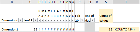
If we didn’t first count the number available, when we try to take ‘n‘ values there may be less than n values for that dimension, resulting in an error.
Step 3: Get the column header of the last value in the row
Having counted the number of available values in each row, it will be useful to know the column header of the latest available value in each row. Because we are using an Excel Table for our source table, we can use structured references (the actual column header) in our formula to retrieve the array of values.
To get the column header, we will:
- look up the last cell in the row that isn’t empty (i.e. not containing a value including zero ‘0’), then
- use ADDRESS and INDIRECT to retrieve the column header for that position.
Find the last non-empty cell in a row
There are several methods in Excel for finding the last value (non-empty) cell in a row or column. The method we’re using is LOOKUP(), and its syntax is shown below. This method can cope with zero values, but not empty cells in the middle of a range:
= LOOKUP(2, 1/(range <> “”), range)
In our example, to find the last cell containing a value in the row of data for Dimension1, the formula would be this if we use cell references:
= LOOKUP(2, 1/(C4:Q4 <> “”), C4:Q4 )
However, as we’re using an Excel Table we can use structured references, where ‘tb_data‘ is the name for our source table, and ‘Jan-19‘ and ‘End of data‘ are the first and last column headers for the range we want Excel to look in:
=LOOKUP(2,1/(tb_data[@[Jan-19]:[End of data]]<>””),tb_data[@[Jan-19]:[End of data]])
HOT TIP:
By using a blank column as the last column in the table, we can add new columns (Mar-20, Apr-20, etc.) before the ‘End of data’ column, and we won’t need to update the lookup formula.
Find the column header for the last non-empty column in the row
Now that we know the last column which contains a value in the row, we use a combination of COLUMN, ADDRESS and INDIRECT to retrieve the actual column header.
Our table headers are in ROW 2 in the Excel worksheet, which we reference in the ADDRESS() function in our formula below.
=INDIRECT(ADDRESS(2,LOOKUP(2,1/(tb_data[@[Jan-19]:[End of data]]<>””),
COLUMN(tb_data[@[Jan-19]:[End of data]]))))
The formula explained
- LOOKUP(2,1/(tb_data[@[Jan-19]:[End of data]]<>””), COLUMN(tb_data[@[Jan-19]:[End of data]]))
- LOOKUP(last non-empty cell),COLUMN(column number of last non-empty cell)
- Adding COLUMN() to the LOOKUP function, returns the column number of the cell containing the last value, not the value itself.
- ADDRESS(2,LOOKUP(2,1/(tb_data[@[Jan-19]:[End of data]]<>””), COLUMN(tb_data[@[Jan-19]:[End of data]])))
- ADDRESS( row 2 [column header row], the column number of the last non-empty cell)
- ADDRESS(rowNumber, colNumber) returns the cell reference of the numbers fed to it.
- We specify ADDRESS(2, colNumber), where the ‘2‘ denotes the second row, and colNumber is the column number we’ve retrieved by combining LOOKUP and COLUMN.
- We wrap the formula inside INDIRECT() which returns the cell contents of the cell reference that it is given.
Summary of the formula
In summary, the formula:
- finds the column number of the last non-empty cell,
- turns the number into a cell reference of type ‘A1’,
- combines it with the row reference of the column headers, and
- feeds the cell reference to INDIRECT which returns the cell’s contents.
Step 4: Retrieve a dynamic array of the latest n values
We are now ready to set up our dynamic array of values in a new table. We’re using the OFFSET() function to set up a range of values to retrieve. OFFSET() takes a starting point, then shifts a number of rows and/or columns relative to the starting point, plus optional height and width of rows and columns to retrieve.
=OFFSET(Reference, Rows, Cols, [height], [width])
OFFSET() function arguments:
- Reference (required): the starting point for the offset. The reference must refer to a cell or range of adjacent cells;
- Rows (required): the number of rows, up or down, relative to the Reference, and can be positive or negative values, e.g.:
- Rows=5, the upper left cell of the target range will be five rows BELOW Reference;
- Rows=-2 (minus 2), the target ranges starts two rows ABOVE Reference
- Rows=0, the upper-left cell is the same as the Reference.
- Cols (required): the number of columns, to the left or right, relative to the Reference. As with the Rows argument above, values can be:
- positive — to the RIGHT of the Reference, or
- negative — to the LEFT of the Reference.
- Height (optional): the number of rows to return; must be a positive number.
- Width (optional): the number of columns, to return; must be a positive number.
In the examples below:
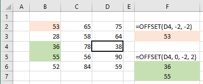
- =OFFSET(D4, -2, -2)
- Reference = D4 (the starting point)
- Rows = -2 (go UP two rows)
- Cols = -2 (go LEFT two columns)
- No other arguments are added, so a single cell’s value is returned.
- =OFFSET(D4, 0, -2, 2)
- Reference = D4 (the starting point)
- Rows = 0 (don’t shift any rows)
- Cols = -2 (go LEFT two columns)
- Height = 2, take cells two rows high.
Key note about OFFSET
The Reference point counts as zero 0. Moving two rows DOWN from D4 takes the upper-left cell of the range to D6 (0=D4, 1 row down=D5, 2 down=D6).
So OFFSET(D3, -3, -3) returns an error value because the cell being referred to does not exist on a worksheet (0=D3, 1 row up=D2, 2 up=D1, 3 up=ERROR, D0 does not exist).
The dynamic array formula
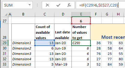
For our dynamic array formula, we’re going to take the column with the latest value (which we found in Step 3), and count back n values.
Using an IF statement we check how many values are available, and retrieve a maximum of 6, but less if fewer are available.
=IF(C29 > 6, $E$27, C29)
=IF(number of values available [C29] > n, select n, else select value in C29). Note that, by entering our desired number of values in cell E27, we can update this value in E27, and the IF formulas referring to E27 will update automatically.
We use INDEX and MATCH to look up the last value in the row for each dimension, and take an array TO THE LEFT of this last value.
Formula in cell F29 in the table below
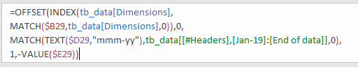
=OFFSET(INDEX(tb_data[Dimensions],MATCH($B29,tb_data[Dimensions],0)),0,MATCH(TEXT($D29,”mmm-yy”),tb_data[[#Headers],[Jan-19]:[End of data]],0),1,-VALUE($E29))
Full dynamic array formula explained
- To run the formula, type it into the cell and with the cursor placed IN THE FORMULA BAR, press Enter (see note below for different actions required according to the version of Excel you are using). Excel will automatically spread the number of values returned into the correct number of cells.
- INDEX(tb_data[Dimensions],MATCH($B29,tb_data[Dimensions],0))
- INDEX MATCH looks in the source data table (tb_data), and finds the row number where ‘Dimension1’ (value in cell B29) appears in the table column [Dimensions]. This becomes the Reference starting point for the OFFSET() function.
- The ‘0’ between the INDEX MATCH and MATCH parts of the formula is the ‘Rows‘ argument for the OFFSET function, and specifies to not shift any rows from the starting row.
- MATCH(TEXT($D29,”mmm-yy”),tb_data[[#Headers],[Jan-19]:[End of data]],0)
- MATCH finds the column number where ‘Jan-20’ (value in cell D29) appears in the table header row.
- OFFSET( …. 1, -VALUE($E29))
- takes the value from INDEX MATCH as the Reference starting point, offsets 0 rows, offsets the number of columns returned from the MATCH function (bullet 3. above), takes 1 row of cells, and the number of columns TO THE LEFT (=minus) specified by the value in cell E29.
Note about Excel versions
- The OFFSET() formula above is an array formula. In the latest version of Excel (2019, Office 365), the formula is run simply by entering the formula, and pressing enter while the cursor is in the formula bar. Excel will automatically enter each value of the array into a cell in the worksheet.
- For older versions of Excel, you need to press Ctrl-Shift-Enter to run the formula (known as an array / CSE formula), but first highlighting the number of cells which will contain the full array.
Step 5: Plot the values in a sparkline chart
Finally, we plot our dynamic array in a sparkline chart.
See our topic page on Excel’s sparklines for how to create, format and clear (delete) sparklines and sparkline groups.
Excel functions and features used to create a dynamic array of values:
- ADDRESS()
- COUNT()
- INDEX()
- INDIRECT()
- LOOKUP()
- MATCH()
- OFFSET()
- TEXT()
- VALUE()
- Excel Table structured references