Purpose: to find where a formula in Excel contains an error, using the EVALUATE FORMULA function, step by step.
If you compile a formula in Excel which results in an error, it is useful to be able to unpick the formula step by step to see at which point the formula is breaking.
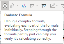
Excel has an inbuilt function — EVALUATE FORMULA — which enables you to do just that.
Links to topics on this page
Where to find the EVALUATE FORMULA command on Excel’s ribbon
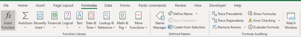
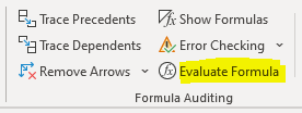
Evaluate Formula is found on the Formulas section of Excel’s ribbon.
TIP: add the command to the quick access toolbar on the ribbon — see our our short video and topic page on how to customize the ribbon in Excel.
Evaluate Formula worked example
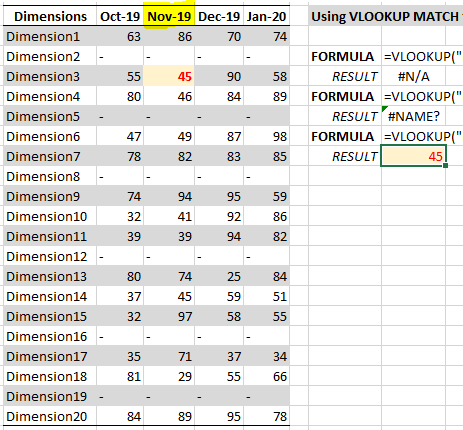
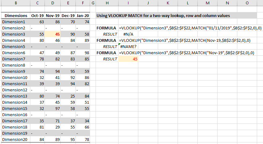
For example, we’re compiling a two-way lookup formula using VLOOKUP and MATCH. The formula is resulting in an error, and we want to see where the error is occurring.
In the example below, we have made two attempts which result in different errors (#N/A and #NAME?), and a third attempt which is successful. We are looking up the value for Dimension3 for Nov-19 (=45).
Method
- Click in the cell containing the formula
- Click on the ‘Evaluate Formula‘ command in the ribbon.
- The Evaluate Formula dialog box opens, displaying the formula.
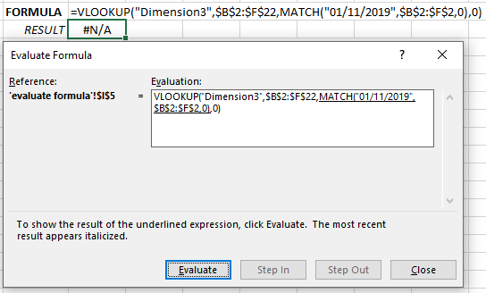
- Now click on the Evaluate button, and Excel takes you through the formula one step at a time. Each click of the button takes you to the next step. You will see where an error appears within the formula. The most recent step result will be in italics.
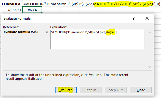
In our example above, there is an error with finding the value “01/11/2019” in the range $B$2:$F$2. The value we’re looking for is November 2019 (entered as Nov-19) and Excel needs us to match the date format exactly.
In the correct formula below, when we use Evaluate Formula to inspect our VLOOKUP MATCH formula, Excel is finding the correct column (Nov-19 is column #3 in our range) to extract the value from.
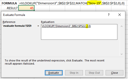
TIP: With VLOOKUP the known value you are using to find the correct row of the target value HAS to be in the left-hand column of the range you are looking in (the ‘Dimensions’ column in our example below). Excel defines this as Column Number 1, and hence our target column for Nov-19 is Column Number 3.