Purpose: create a row by row list to keep track of rows and stitches in a knitting pattern in Excel.
In this post we get back to basics with a simple practical example.
Here’s how to use an Excel spreadsheet to create a tick list of rows and stitch counts for a knitting pattern.
We’re going to use the basic functions of:
- copy and paste,
- flash fill,
- running total, and
- rotate text for adjusting layout to fit your print page size.
Links to topics on this page
- Create column headings;
- Flash fill row cell contents down a column;
- Add row instructions, highlight and repeat cells;
- Add the running total formula and flash fill down;
- View the print preview;
- Rotate text;
- Related topics.
Worked example
In a knitting pattern, we often see a summary of instructions, for example, decreasing for shaping armholes or shoulders as below:
Shape Raglan Armholes:
- Cast off 3 sts at beg of next 2 rows. 85 [91: 97: 103: 109: 115] sts.
- Dec 1 st at each end of next and 11 [9: 8: 6: 5: 2] foll 4th rows,
- then on foll 16 [20: 24: 28: 32: 38] alt rows. 29 [31: 31: 33: 33: 33] sts.
- Work 1 row, ending with a ws row. Break yarn and leave sts on a holder.
Based on this summary above, we’re going to create a tick list of row instructions which will help us to keep track of rows and stitch numbers. This will be much quicker than creating a handwritten list, and more reliable than simply keeping a written tally of counts.
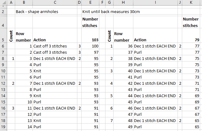
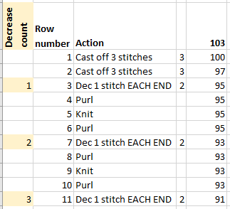
We want to create a list like the one below:
| Decrease count | Row number | Action | Stitch decrease | Running total |
| 1 | 3 | Dec 1 stitch each end | 2 | 95 |
| 4 | Purl | 0 | 95 |
Create column headings
In a blank worksheet, type in your column headings, e.g.
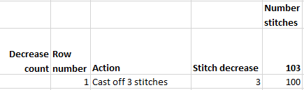
- Decrease count (a tally of the number of times the decrease row needs to be repeated)
- Row number
- Action (e.g. knit, purl, decrease 1 stitch each end)
- Stitch decrease (number of stitches which are decreased in the row). This column will be used in our running total calculation.
- Number stitches (the running total of stitches).
Flash fill the row number down the column
Type in the number 1 into the first cell under the ‘Row number’ heading.
The row number increments by one each row, so having typed in 1 into the first row, we can use Excel’s flash fill function to add the row numbers down the column as required.
- Click on the cell where you’ve typed ‘1’, and then click and drag down the right-hand bottom corner of the cell.
- Excel will copy the contents down the column as far as you drag the mouse.
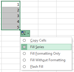
- When you release the mouse, the new cells remain highlighted and the ‘Auto fill options‘ icon is available.
- Click on the icon, and select ‘Fill Series’ from the options.
- The cells will now be filled with an increasing list of row numbers, incrementing by 1.
Add row instructions, highlight and repeat down the column
Here we need to add just enough details that we can then copy and paste down the sheet.
We describe two methods below for repeating a range of cells down a column:
Method 1: Use flash fill to repeat cells down a column
- Select the range of cells to repeat down the column. The cells can extend over more than one column.
- With the cells now selected and highlighted, click on the bottom right-hand corner of the cell range, and drag down the column. The cells will be repeated, as far as you drag.
- NOTE: The cells remain highlighted after you release the mouse. However, if you attempt to amend your intended repetition by clicking and dragging the corner again, you may find that the cell range being repeated isn’t quite what you expect!
Method 2: Copy and paste a range of cells down a column
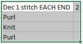
- Type in the repeating sequence of rows (one decrease row instruction, and type 2 in the ‘Decrease stitches‘ column, followed by 3 rows of Purl, Knit, Purl). The pattern instruction is: Dec 1 st at each end of next and 11 [9: 8: 6: 5: 2] foll 4th rows.
- Highlight the cells (click in one corner cell, and drag the mouse to cover all the cells to copy). Copy using your preferred method (press Ctrl-C on the keyboard; or right-click and select Copy; or select Copy from the Home | Clipboard menu).
- Click in the cell below your last row entry, and select Paste (Ctrl-V on the keyboard; or right-click and select Paste; or select Paste from the Home | Clipboard menu).
- TIP: The copied cells remain in the clipboard, so you can paste as many times as the rows need to be repeated (9,8,6,5, or 2 from the pattern instruction in step 1), repeating step 3. above.
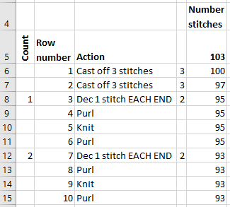
We use the ‘Decrease count‘ column to count the number of repeats of the decrease sequence of rows.
Add the running total formula and flash fill down
We now add the simple running total formula to automatically update the count of stitches remaining on the needles.
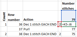
The formula to keep the tally of stitches is the number of stitches in the previous row, minus the number to decrease:
= K5 – J6
Enter this formula into the cell below the start number of stitches. As before, flash fill this formula down the ‘Number stitches‘ column, and the running total of stitches will be calculated.
Using the simple steps above, we can quickly create a row by row tick list to follow for knitting the pattern.
View the print preview
When we’re ready to print, we can view the print preview to check that we can fit our list neatly on to A4 sheet(s).
To view print preview you have various options:
- Select File | Print, or press Ctrl-P. The print options and preview are displayed;
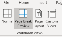
- Click on the Page Break Preview icon at the bottom of each worksheet. To return to the normal grid worksheet view, click on the squared Normal icon;
- Select Page Break Preview from the Workbook Views section on the Views tab of the ribbon.
Rotate text in column headings
One way to reduce the widths of columns, is to rotate the text in the column header.
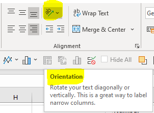
Click in the column header cell to select the cell, and click on the Orientation icon in the Home | Alignment section of the ribbon. There are many options to choose from:
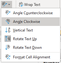
As Excel says, “This is a great way to label narrow columns.” 🙂
When you’re happy with the layout, you are ready to print your finished list: