Purpose

Create a list of items which can be selected from a dropdown selector in a cell, using data validation

---

Links to topics on this page

• Add a dropdown list
• Clear data validation from a cell
• Create a named range in Excel

---

Method — add a dropdown list to a cell in Excel and copy data validation to other cells

• First create your list(s) of items that are to be chosen from, in separate columns (or in separate ranges). The lists can be on the same worksheet, or another worksheet.
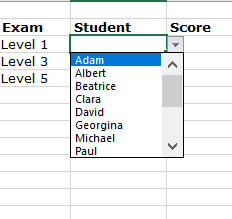
• In the video example we have created a list of exam names and student names.
• To make it easier to refer to the lists (especially if they are on a different worksheet), and to add additional items to the lists, name the lists via the ‘Name manager‘ feature in Excel.
• If you don’t yet know how to name a range of cells, see the quick help below.
• The video above shows how to add a dropdown list to a cell, and different ways to copy the dropdown selector to another cell, or range of cells.

1. Select the cell/range of cells that you would like the dropdown list to be selected from.
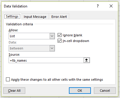
2. Click on the ‘Data validation‘ option from the Data tab | Data tools section of the ribbon.
3. In the ‘Data Validation’ dialog box, enter ‘=‘ followed by the named range of cells that contains the list (in the screenshot above, the range is called ‘tb_names‘). Click OK.
4. You will now see that a dropdown arrow appears at the right-hand edge of the cell, and when you click on it, your dropdown list can be selected from.
5. To copy the selector to another cell:
   • Copy the cell with the dropdown. Select the cell, or range of cells to copy to, right-click, and select ‘Paste Special…’. In the Paste Special dialog box, check the radio button next to ‘Validation’. The dropdown list will now be available from the cell(s).
   • Or, if you want to copy the cells to adjacent cells down a column, select the cell with the dropdown selector, and drag the right-hand corner of the cell down the column.

Method — to clear data validation from a cell

Select the cell with the dropdown selector, and open the ‘Data Validation’ dialog box from the ribbon. Click on the ‘Clear all’ button at the bottom of the dialog box.

Method — to create a ‘named’ range of cells in Excel

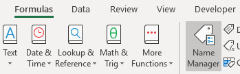
Select the range of cells to be named, and from the Formulas tab, click on the ‘Name Manager‘ icon. (Note — you don’t have to select the cells first, you can open the Name Manager dialog box first, and add your cell range in a later step.)

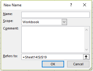
In the Name Manager dialog box, click on ‘New‘, and the ‘New name‘ dialog box opens. Enter a name for your range, add or adjust the range of cells as required, and click OK.

To edit the range of cells, use the Name Manager again to adjust the cells included in the range.