Purpose
Add a reference line, such as an average or benchmark, to a vertical bar chart in Excel.
Method – example adding an average line (see video below)

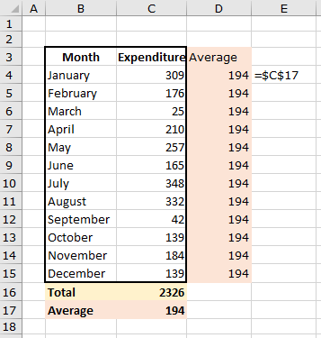
- Add a ‘helper column’ – calculate the average, and add this value to the column next to your main data
- Click on the chart to select it, and from the Design tab, click on the ‘Select Data‘ icon.
- In the left hand pane (Legend Entries (Series)), click on the Add icon, and in the popup window, select the column header of your helper column, for the series name, and the column of values for the series values.
- The bars for the average values will be added to the chart.
- Click on one of the bars for the average values, and right-click. Select ‘Change series chart type‘.
- From the Chart type dropdown next to the Average series name, select ‘Line‘. The average values will now be displayed as a horizontal line across the chart.

