PURPOSE

To test IF a value matches a condition, and return one result if TRUE, and another if FALSE.

SYNTAX | EXAMPLE

=IF(A2=[condition],Return1,Return2)

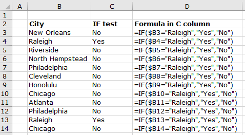
=IF($B3=”Raleigh”,”Yes”,”No”)

EXPLANATION of example below

The Excel IF function looks in cell B3 and if it contains the word “Raleigh” then it will return the first value (“Yes”); if B3 doesn’t contain “Raleigh” it will return the second value (“No”). The match is NOT case sensitive, so a ‘Yes’ would be returned if the search word was “raleigh”.

Conditional formatting – highlight cells with a specific value

View the short video below on how to highlight the ‘Yes’ values in the ‘IF test’ column, using Excel’s Conditional Formatting to create a conditional formatting ‘rule’.

1. Click and drag over the range of cells to apply the conditional formatting rule to.
2. From the ‘Styles‘ section in the ribbon, click on:
   1. Conditional Formatting
   2. Highlight Cells Rules,
   3. Text that contains.
3. In the popup box, enter the Text to search for, in our example ‘Yes’, and select the styling to highlight the values with – one of the pre-formatted options, or a custom format.
4. Click OK.
5. You can amend the rule options by clicking back on Conditional Formatting, and select ‘Manage rules‘.